라운드 로빈 각 프로세스에 고정된 시간 슬롯이 주기적으로 할당되는 CPU 스케줄링 알고리즘입니다. 이는 선착순 CPU 스케줄링 알고리즘의 선점형 버전입니다.
김프 배경 삭제
- 라운드 로빈 CPU 알고리즘은 일반적으로 시간 공유 기술에 중점을 둡니다.
- 프로세스나 작업이 선점형 방식으로 실행되도록 허용되는 기간을 시간이라고 합니다. 양자 .
- 준비 대기열에 있는 각 프로세스나 작업에는 해당 시간 할당량에 대한 CPU가 할당됩니다. 해당 시간 동안 프로세스 실행이 완료되면 프로세스는 끝 그렇지 않으면 프로세스가 이전 단계로 되돌아갑니다. 대기 테이블 실행을 완료하기 위해 다음 차례를 기다립니다.
Round Robin CPU 스케줄링 알고리즘의 특징
- 모든 프로세스가 CPU를 공평하게 공유하므로 간단하고 구현하기 쉬우며 기아 현상이 없습니다.
- 에서 가장 일반적으로 사용되는 기술 중 하나 CPU 스케줄링 핵심이다.
- 그것은 선제적인 프로세스에는 최대 고정된 시간 동안만 CPU가 할당되기 때문입니다.
- 단점은 컨텍스트 전환에 따른 오버헤드가 더 크다는 것입니다.
라운드 로빈 CPU 스케줄링 알고리즘의 장점
- 모든 프로세스가 CPU를 동일하게 공유하므로 공정성이 있습니다.
- 새로 생성된 프로세스는 준비 대기열의 끝에 추가됩니다.
- 라운드 로빈 스케줄러는 일반적으로 시간 공유를 사용하여 각 작업에 시간 슬롯 또는 할당량을 제공합니다.
- 라운드 로빈 스케줄링을 수행하는 동안 특정 시간 할당량이 다른 작업에 할당됩니다.
- 각 프로세스는 이 스케줄링에서 특정 양자 시간 이후에 일정을 다시 잡을 수 있는 기회를 얻습니다.
라운드 로빈 CPU 스케줄링 알고리즘의 단점
- 대기 시간과 응답 시간이 더 큽니다.
- 처리량이 낮습니다.
- 컨텍스트 스위치가 있습니다.
- 간트 차트가 너무 큰 것 같습니다(스케줄링에 대한 양자 시간이 더 적은 경우. 예: 대규모 스케줄링의 경우 1ms.)
- 작은 양자에 대한 시간 소모적인 스케줄링.
작업을 보여주는 예 라운드 로빈 스케줄링 알고리즘
예-1: 4개 프로세스의 도착 시간과 버스트 시간에 대한 다음 표를 고려하세요. P1, P2, P3, P4 그리고 주어진 시간 퀀텀 = 2
| 프로세스 | 버스트 시간 | 도착 시간 |
|---|---|---|
| P1 | 5ms | 0ms |
| P2 | 4ms | 1ms |
| P3 | 2ms | 2ms |
| P4 | 1ms | 4ms |
라운드 로빈 CPU 스케줄링 알고리즘은 아래 언급된 단계를 기반으로 작동합니다.
시간 = 0,
- 실행은 버스트 시간이 5인 프로세스 P1에서 시작됩니다.
- 여기서 모든 프로세스는 2밀리초 동안 실행됩니다( 시간양자주기 ). P2와 P3은 아직 대기 대기열에 있습니다.
| 시간 인스턴스 | 프로세스 | 도착 시간 | 준비 대기열 | 실행 중인 대기열 | 실행 시간 | 초기 버스트 시간 | 남은 버스트 시간 |
|---|---|---|---|---|---|---|---|
| 0-2ms | P1 | 0ms | P2, P3 | P1 | 2ms | 5ms | 3ms |
시간 = 2,
- 프로세스 P1과 P3은 준비 대기열에 도착하고 P2는 실행을 시작합니다. TQ 기간
| 시간 인스턴스 | 프로세스 | 도착 시간 | 준비 대기열 | 실행 중인 대기열 | 실행 시간 | 초기 버스트 시간 | 남은 버스트 시간 |
|---|---|---|---|---|---|---|---|
| 2-4ms | P1 | 0ms | P3, P1 | P2 | 0ms | 3ms | 3ms |
| P2 | 1ms | 2ms | 4ms | 2ms |
시간 = 4,
- 프로세스 P4가 준비 대기열 ,
- 그런 다음 P3이 실행됩니다. TQ 기간.
| 시간 인스턴스 | 프로세스 | 도착 시간 | 준비 대기열 | 실행 중인 대기열 | 실행 시간 | 초기 버스트 시간 | 남은 버스트 시간 |
|---|---|---|---|---|---|---|---|
| 4-6ms | P1 | 0ms | P1, P4, P2 | P3 | 0ms | 3ms | 3ms |
| P2 | 1ms | 0ms | 2ms | 2ms | |||
| P3 | 2ms | 2ms | 2ms | 0ms |
시간 = 6,
- 프로세스 P3이 실행을 완료합니다.
- 프로세스 P1이 다음에 대해 실행을 시작합니다. TQ b의 다음 기간과 같습니다.
| 시간 인스턴스 | 프로세스 | 도착 시간 | 준비 대기열 | 실행 중인 대기열 | 실행 시간 | 초기 버스트 시간 | 남은 버스트 시간 |
|---|---|---|---|---|---|---|---|
| 6-8ms | P1 | 0ms | P4, P2 | P1 | 2ms | 3ms | 1ms |
| P2 | 1ms | 0ms | 2ms | 2ms |
시간 = 8,
- 프로세스 P4가 실행을 시작하지만 다음 기간 동안 실행되지 않습니다. 시간양자주기 버스트 시간 = 1이므로
- 따라서 1ms 동안만 실행됩니다.
| 시간 인스턴스 | 프로세스 | 도착 시간 | 준비 대기열 | 실행 중인 대기열 | 실행 시간 | 초기 버스트 시간 | 남은 버스트 시간 |
|---|---|---|---|---|---|---|---|
| 8-9ms | P1 | 0ms | P2, P1 | P4 | 0ms | 3ms | 1ms |
| P2 | 1ms | 0ms | 2ms | 2ms | |||
| P4 | 4ms | 1ms | 1ms | 0ms |
시간 = 9,
- 프로세스 P4가 실행을 완료합니다.
- 프로세스 P2가 다음에 대해 실행을 시작합니다. TQ 기간은 다음과 같습니다. 준비 대기열
| 시간 인스턴스 | 프로세스 | 도착 시간 | 준비 대기열 | 실행 중인 대기열 | 실행 시간 | 초기 버스트 시간 | 남은 버스트 시간 |
|---|---|---|---|---|---|---|---|
| 9-11ms | P1 | 0ms | P1 | P2 | 0ms | 3ms | 1ms |
| P2 | 1ms | 2ms | 2ms | 0ms |
시간 = 11,
- 프로세스 P2가 실행을 완료합니다.
- 프로세스 P1이 실행을 시작하고 1ms 동안만 실행됩니다.
| 시간 인스턴스 | 프로세스 | 도착 시간 | 준비 대기열 | 실행 중인 대기열 | 실행 시간 | 초기 버스트 시간 | 남은 버스트 시간 |
|---|---|---|---|---|---|---|---|
| 11-12ms | P1 | 0ms | P1 | 1ms | 1ms | 0ms |
시간 = 12,
- 프로세스 P1이 실행을 완료합니다.
- 프로세스의 전반적인 실행은 다음과 같습니다.
| 시간 인스턴스 | 프로세스 | 도착 시간 | 준비 대기열 | 실행 중인 대기열 | 실행 시간 | 초기 버스트 시간 | 남은 버스트 시간 |
|---|---|---|---|---|---|---|---|
| 0-2ms | P1 | 0ms | P2, P3 | P1 | 2ms | 5ms | 3ms |
| 2-4ms | P1 | 0ms | P3, P1 | P2 | 0ms | 3ms | 3ms |
| P2 | 1ms | 2ms | 4ms | 2ms | |||
| 4-6ms | P1 | 0ms | P1, P4, P2 | P3 | 0ms | 3ms | 3ms |
| P2 | 1ms | 0ms | 2ms | 2ms | |||
| P3 | 2ms | 2ms | 2ms | 0ms | |||
| 6-8ms | P1 | 0ms | P4, P2 | P1 | 2ms | 3ms | 1ms |
| P2 | 1ms | 0ms | 2ms | 2ms | |||
| 8-9ms | P1 | 0ms | P2, P1 | P4 | 0ms | 3ms | 1ms |
| P2 | 1ms | 0ms | 2ms | 2ms | |||
| P4 | 4ms | 1ms | 1ms | 0ms | |||
| 9-11ms | P1 | 0ms | P1 | P2 | 0ms | 3ms | 1ms |
| P2 | 1ms | 2ms | 2ms | 0ms | |||
| 11-12ms | P1 | 0ms | P1 | 1ms | 1ms | 0ms |
간트 차트 아래와 같이 됩니다.
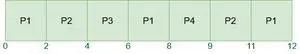
라운드 로빈 스케줄링 알고리즘에 대한 간트 차트
프로그램을 사용하여 라운드 로빈에서 아래 시간을 계산하는 방법은 무엇입니까?
- 완료 시간: 프로세스가 실행을 완료하는 시간입니다.
- 처리 시간: 시간 완료 시간과 도착 시간의 차이입니다. 처리 시간 = 완료 시간 – 도착 시간
- 대기 시간(W.T): 시간 처리 시간과 버스트 시간의 차이입니다.
대기 시간 = 처리 시간 – 버스트 시간
이제 평균을 계산해보자 기다리는 시간과 돌아서 시간:
| 프로세스 | 에 | 비티 | CT | 싸구려 | WT |
|---|---|---|---|---|---|
| P1 | 0 | 5 | 12 | 12-0 = 12 | 12-5 = 7 |
| P2 | 1 | 4 | 열하나 | 11-1 = 10 | 10-4 = 6 |
| P3 | 2 | 2 | 6 | 6-2 = 4 | 4-2 = 2 |
| P4 | 4 | 1 | 9 | 9-4 = 5 | 5-1 = 4 |
지금,
- 평균 처리 시간 = (12 + 10 + 4 + 5)/4 = 31/4 = 7.7
- 평균 대기 시간 = (7 + 6 + 2 + 4)/4 = 19/4 = 4.7
예시 2: 세 가지 프로세스 P1, P2, P3에 대한 도착 시간과 버스트 시간에 대한 다음 표를 고려하십시오. 시간 퀀텀 = 2
| 프로세스 | 버스트 시간 | 도착 시간 |
|---|---|---|
| P1 | 10ms | 0ms |
| P2 | 5ms | 0ms |
| P3 | 8ms | 0ms |
비슷하게, 간트 차트 이 예의 경우:

예 2의 간트 차트
이제 평균을 계산해보자 기다리는 시간과 돌아서 시간:
| 프로세스 | 에 | 비티 | CT | 싸구려 | WT |
|---|---|---|---|---|---|
| P1 | 0 | 10 | 23 | 23-0 = 23 | 23-10 = 13 |
| P2 | 0 | 5 | 열 다섯 | 15-0 = 15 | 15-5 = 10 |
| P3 | 0 | 8 | 이십 일 | 21-0 = 21 | 21-8 = 13 |
총 처리 시간 = 59ms
그래서, 평균 처리 시간 = 59/3 = 19.667ms그리고 총 대기 시간 = 36ms
그래서, 평균 대기 시간 = 36/3 = 12.00ms
모든 프로세스에 대해 도착 시간을 0으로 하는 라운드 로빈 스케줄링 프로그램
모든 프로세스의 대기 시간을 찾는 단계
- 배열 만들기 rem_bt[] 프로세스의 남은 버스트 시간을 추적합니다. 이 배열은 처음에는 bt[](버스트 시간 배열)의 복사본입니다.
- 다른 어레이 생성 중량[] 프로세스의 대기 시간을 저장합니다. 이 배열을 0으로 초기화합니다.
- 초기화 시간 : t = 0
- 완료되지 않은 동안 모든 프로세스를 계속 순회합니다. 다음을 수행하십시오. 나는 아직 완료되지 않은 경우 처리합니다.
- rem_bt[i]> 양자인 경우
- t = t + 양자
- rem_bt[i] -= 금액;
- Else // 이 프로세스의 마지막 주기
- t = t + rem_bt[i];
- 중량[i] = t - bt[i]
- rem_bt[i] = 0; // 이 과정은 끝났습니다
대기 시간이 있으면 프로세스의 처리 시간 tat[i]를 대기 시간과 버스트 시간의 합으로 계산할 수 있습니다(즉, wt[i] + bt[i]).
다음은 위 단계의 구현입니다.
C++
자바 스위치
// C++ program for implementation of RR scheduling> #include> using> namespace> std;> // Function to find the waiting time for all> // processes> void> findWaitingTime(>int> processes[],>int> n,> >int> bt[],>int> wt[],>int> quantum)> {> >// Make a copy of burst times bt[] to store remaining> >// burst times.> >int> rem_bt[n];> >for> (>int> i = 0 ; i rem_bt[i] = bt[i]; int t = 0; // Current time // Keep traversing processes in round robin manner // until all of them are not done. while (1) { bool done = true; // Traverse all processes one by one repeatedly for (int i = 0 ; i { // If burst time of a process is greater than 0 // then only need to process further if (rem_bt[i]>0) { 완료 = 거짓; // 보류 중인 프로세스가 있습니다. if (rem_bt[i]> Quantum) { // t의 값을 늘립니다. 즉 // 프로세스가 처리된 시간을 표시합니다. t += Quantum; // 현재 프로세스의 버스트 시간을 // 퀀텀만큼 줄입니다. rem_bt[i] -= 퀀텀; } // 버스트 시간이 퀀텀보다 작거나 같은 경우 //. 이 프로세스의 마지막 주기 else { // t의 값을 늘립니다. 즉 // 프로세스가 처리된 시간을 보여줍니다. t = t + rem_bt[i]; // 대기 시간은 현재 시간에서 // 이 프로세스에 사용되는 시간입니다. wt[i] = t - bt[i]; // 프로세스가 완전히 실행되면 // 남은 버스트 시간을 0으로 만듭니다. rem_bt[i] = 0; } } } // 모든 프로세스가 완료되면 if (done == true) break; } } // 소요 시간을 계산하는 함수 void findTurnAroundTime(int process[], int n, int bt[], int wt[], int tat[]) { // bt[i]를 더하여 // 소요 시간을 계산합니다. + wt[i] for (int i = 0; i tat[i] = bt[i] + wt[i]; } // 평균 시간을 계산하는 함수 void findavgTime(int process[], int n, int bt[ ], int Quantum) { int wt[n], tat[n], total_wt = 0, total_tat = 0; // 모든 프로세스의 대기 시간을 구하는 함수 findWaitingTime(processes, n, bt, wt, Quantum); 모든 프로세스의 처리 시간을 찾는 함수 findTurnAroundTime(processes, n, bt, wt, tat) // 모든 세부 정보와 함께 프로세스를 표시합니다.<< 'PN '<< ' BT ' << ' WT ' << ' TAT
'; // Calculate total waiting time and total turn // around time for (int i=0; i { total_wt = total_wt + wt[i]; total_tat = total_tat + tat[i]; cout << ' ' << i+1 << ' ' << bt[i] <<' ' << wt[i] <<' ' << tat[i] < } cout << 'Average waiting time = ' << (float)total_wt / (float)n; cout << '
Average turn around time = ' << (float)total_tat / (float)n; } // Driver code int main() { // process id's int processes[] = { 1, 2, 3}; int n = sizeof processes / sizeof processes[0]; // Burst time of all processes int burst_time[] = {10, 5, 8}; // Time quantum int quantum = 2; findavgTime(processes, n, burst_time, quantum); return 0; }> |
>
>
자바
// Java program for implementation of RR scheduling> public> class> GFG> {> >// Method to find the waiting time for all> >// processes> >static> void> findWaitingTime(>int> processes[],>int> n,> >int> bt[],>int> wt[],>int> quantum)> >{> >// Make a copy of burst times bt[] to store remaining> >// burst times.> >int> rem_bt[] =>new> int>[n];> >for> (>int> i =>0> ; i rem_bt[i] = bt[i]; int t = 0; // Current time // Keep traversing processes in round robin manner // until all of them are not done. while(true) { boolean done = true; // Traverse all processes one by one repeatedly for (int i = 0 ; i { // If burst time of a process is greater than 0 // then only need to process further if (rem_bt[i]>0) { 완료 = 거짓; // 보류 중인 프로세스가 있습니다. if (rem_bt[i]> Quantum) { // t의 값을 늘립니다. 즉 // 프로세스가 처리된 시간을 표시합니다. t += Quantum; // 현재 프로세스의 버스트 시간을 // 퀀텀만큼 줄입니다. rem_bt[i] -= 퀀텀; } // 버스트 시간이 퀀텀보다 작거나 같은 경우 //. 이 프로세스의 마지막 주기 else { // t의 값을 늘립니다. 즉 // 프로세스가 처리된 시간을 보여줍니다. t = t + rem_bt[i]; // 대기 시간은 현재 시간에서 // 이 프로세스에 사용되는 시간입니다. wt[i] = t - bt[i]; // 프로세스가 완전히 실행되면 // 남은 버스트 시간을 0으로 만듭니다. rem_bt[i] = 0; } } } // 모든 프로세스가 완료되면 if (done == true) break; } } // 소요 시간을 계산하는 방법 static void findTurnAroundTime(int process[], int n, int bt[], int wt[], int tat[]) { // bt[i를 더하여 // 소요 시간을 계산합니다. ] + wt[i] for (int i = 0; i tat[i] = bt[i] + wt[i]; } // 평균 시간을 계산하는 방법 static void findavgTime(int process[], int n, int bt[], int Quantum) { int wt[] = new int[n], tat[] = new int[n]; int total_wt = 0, total_tat = 0; // 모든 프로세스의 대기시간을 구하는 함수 findWaitingTime( processs, n, bt, wt, Quantum); // 모든 프로세스의 처리 시간을 찾는 함수 findTurnAroundTime(processes, n, bt, wt, tat) // 모든 세부 정보와 함께 프로세스 표시 System.out.println( 'PN ' + ' B ' + ' WT ' + ' TAT'); // 총 대기 시간과 총 회전 시간을 // 계산합니다 for (int i=0; i { total_wt = total_wt + wt[i]; total_tat = total_tat + tat[i]; System.out.println(' ' + (i+1) + ' ' + bt[i] +' ' + wt[i] +' ' + tat[i]); } System.out.println('평균 대기 시간 = ' + (float)total_wt / (float)n); System.out.println('평균 처리 시간 = ' + (float)total_tat / (float)n); } // 드라이버 메서드 public static void main(String[] args) { // 프로세스 ID의 int process[] = { 1, 2, 3}; int n = 프로세스.길이; // 모든 프로세스의 버스트 시간 int Burst_time[] = {10, 5, 8}; // 시간 퀀텀 int 퀀텀 = 2; findavgTime(프로세스, n, 버스트_시간, 양자); } }> |
>
>
파이썬3
봄의 JPA
# Python3 program for implementation of> # RR scheduling> # Function to find the waiting time> # for all processes> def> findWaitingTime(processes, n, bt,> >wt, quantum):> >rem_bt>=> [>0>]>*> n> ># Copy the burst time into rt[]> >for> i>in> range>(n):> >rem_bt[i]>=> bt[i]> >t>=> 0> # Current time> ># Keep traversing processes in round> ># robin manner until all of them are> ># not done.> >while>(>1>):> >done>=> True> ># Traverse all processes one by> ># one repeatedly> >for> i>in> range>(n):> > ># If burst time of a process is greater> ># than 0 then only need to process further> >if> (rem_bt[i]>>0>) :> >done>=> False> # There is a pending process> > >if> (rem_bt[i]>양자) :> > ># Increase the value of t i.e. shows> ># how much time a process has been processed> >t>+>=> quantum> ># Decrease the burst_time of current> ># process by quantum> >rem_bt[i]>->=> quantum> > ># If burst time is smaller than or equal> ># to quantum. Last cycle for this process> >else>:> > ># Increase the value of t i.e. shows> ># how much time a process has been processed> >t>=> t>+> rem_bt[i]> ># Waiting time is current time minus> ># time used by this process> >wt[i]>=> t>-> bt[i]> ># As the process gets fully executed> ># make its remaining burst time = 0> >rem_bt[i]>=> 0> > ># If all processes are done> >if> (done>=>=> True>):> >break> > # Function to calculate turn around time> def> findTurnAroundTime(processes, n, bt, wt, tat):> > ># Calculating turnaround time> >for> i>in> range>(n):> >tat[i]>=> bt[i]>+> wt[i]> # Function to calculate average waiting> # and turn-around times.> def> findavgTime(processes, n, bt, quantum):> >wt>=> [>0>]>*> n> >tat>=> [>0>]>*> n> ># Function to find waiting time> ># of all processes> >findWaitingTime(processes, n, bt,> >wt, quantum)> ># Function to find turn around time> ># for all processes> >findTurnAroundTime(processes, n, bt,> >wt, tat)> ># Display processes along with all details> >print>(>'Processes Burst Time Waiting'>,> >'Time Turn-Around Time'>)> >total_wt>=> 0> >total_tat>=> 0> >for> i>in> range>(n):> >total_wt>=> total_wt>+> wt[i]> >total_tat>=> total_tat>+> tat[i]> >print>(>' '>, i>+> 1>,>' '>, bt[i],> >' '>, wt[i],>' '>, tat[i])> >print>(>'
Average waiting time = %.5f '>%>(total_wt>/>n) )> >print>(>'Average turn around time = %.5f '>%> (total_tat>/> n))> > # Driver code> if> __name__>=>=>'__main__'>:> > ># Process id's> >proc>=> [>1>,>2>,>3>]> >n>=> 3> ># Burst time of all processes> >burst_time>=> [>10>,>5>,>8>]> ># Time quantum> >quantum>=> 2>;> >findavgTime(proc, n, burst_time, quantum)> # This code is contributed by> # Shubham Singh(SHUBHAMSINGH10)> |
>
>
씨#
// C# program for implementation of RR> // scheduling> using> System;> public> class> GFG {> > >// Method to find the waiting time> >// for all processes> >static> void> findWaitingTime(>int> []processes,> >int> n,>int> []bt,>int> []wt,>int> quantum)> >{> > >// Make a copy of burst times bt[] to> >// store remaining burst times.> >int> []rem_bt =>new> int>[n];> > >for> (>int> i = 0 ; i rem_bt[i] = bt[i]; int t = 0; // Current time // Keep traversing processes in round // robin manner until all of them are // not done. while(true) { bool done = true; // Traverse all processes one by // one repeatedly for (int i = 0 ; i { // If burst time of a process // is greater than 0 then only // need to process further if (rem_bt[i]>0) { // 보류 중인 프로세스가 있습니다. done = false; if (rem_bt[i]> Quantum) { // t의 값을 늘립니다. 즉, // 프로세스가 처리된 시간을 // 표시합니다. t += Quantum; // 현재 프로세스의 //burst_time을 퀀텀으로 줄입니다. rem_bt[i] -= 퀀텀; } // 버스트 시간이 퀀텀보다 // 작거나 같은 경우. // 이 프로세스의 마지막 사이클 else { // t의 값을 늘립니다. 즉 // 프로세스가 처리된 시간을 // 보여줍니다. t = t + rem_bt[i]; // 대기 시간은 현재 // 시간에서 // 이 프로세스에 사용된 시간을 뺀 것입니다. wt[i] = t - bt[i]; // 프로세스가 완전히 실행되면 // 남은 시간을 버스트 시간 = 0으로 만듭니다. rem_bt[i] = 0; } } } // 모든 프로세스가 완료되면 if (done == true) break; } } // 소요 시간을 계산하는 방법 static void findTurnAroundTime(int []processes, int n, int []bt, int []wt, int []tat) { // bt[i를 더하여 // 소요 시간을 계산합니다. ] + wt[i] for (int i = 0; i tat[i] = bt[i] + wt[i]; } // 평균 시간을 계산하는 방법 static void findavgTime(int []processes, int n, int []bt, int Quantum) { int []wt = new int[n]; int []tat = new int[n] int total_wt = 0, total_tat = 0; // 전체의 대기 시간을 구하는 함수 process findWaitingTime(processes, n, bt, wt, Quantum); // 모든 프로세스에 대한 처리 시간을 찾는 함수 findTurnAroundTime(processes, n, bt, wt, tat) // 모든 세부 사항과 함께 프로세스 표시 Console.WriteLine('프로세스 ' + ' 버스트 시간 ' + ' 대기 시간 ' + ' 처리 시간') // 총 대기 시간 및 총 회전 시간 계산 for (int i = 0; i { total_wt = total_wt + wt[i]; total_tat = total_tat + tat[i] Console.WriteLine(' ' + (i+1) + ' ' + bt[i ] + ' ' + wt[i] +' ' + tat[i]); } Console.WriteLine('평균 대기 시간 = ' + (float)total_wt / (float)n); Console.Write('평균 처리 시간 = ' + (float)total_tat / (float)n); } // 드라이버 메서드 public static void Main() { // 프로세스 ID의 int []processes = { 1, 2, 3}; int n = 프로세스.길이; // 모든 프로세스의 버스트 시간 int []burst_time = {10, 5, 8}; // 시간 퀀텀 int 퀀텀 = 2; findavgTime(프로세스, n, 버스트_시간, 양자); } } // 이 코드는 nitin mittal이 제공한 것입니다.> |
>
>
자바스크립트
> >// JavaScript program for implementation of RR scheduling> >// Function to find the waiting time for all> >// processes> >const findWaitingTime = (processes, n, bt, wt, quantum) =>{> >// Make a copy of burst times bt[] to store remaining> >// burst times.> >let rem_bt =>new> Array(n).fill(0);> >for> (let i = 0; i rem_bt[i] = bt[i]; let t = 0; // Current time // Keep traversing processes in round robin manner // until all of them are not done. while (1) { let done = true; // Traverse all processes one by one repeatedly for (let i = 0; i // If burst time of a process is greater than 0 // then only need to process further if (rem_bt[i]>0) { 완료 = 거짓; // 보류 중인 프로세스가 있습니다. if (rem_bt[i]> Quantum) { // t의 값을 늘립니다. 즉 // 프로세스가 처리된 시간을 표시합니다. t += Quantum; // 현재 프로세스의 버스트 시간을 // 퀀텀만큼 줄입니다. rem_bt[i] -= 퀀텀; } // 버스트 시간이 퀀텀보다 작거나 같은 경우 //. 이 프로세스의 마지막 주기 else { // t의 값을 늘립니다. 즉 // 프로세스가 처리된 시간을 보여줍니다. t = t + rem_bt[i]; // 대기 시간은 현재 시간에서 // 이 프로세스에 사용되는 시간입니다. wt[i] = t - bt[i]; // 프로세스가 완전히 실행되면 // 남은 버스트 시간을 0으로 만듭니다. rem_bt[i] = 0; } } } // 모든 프로세스가 완료되면 if (done == true) break; } } // 처리 시간을 계산하는 함수 const findTurnAroundTime = (processes, n, bt, wt, tat) => { // bt[i] + wt[i] for (let i = 0; i tat[i] = bt[i] + wt[i]; } // 평균 시간을 계산하는 함수 const findavgTime = (processes, n, bt, Quantum) => { let wt = new Array(n). fill(0), tat = new Array(n).fill(0); let total_wt = 0, total_tat = 0; // 모든 프로세스의 대기 시간을 구하는 함수 findWaitingTime(processes, n, bt, wt, Quantum); // 모든 프로세스에 대한 처리 시간을 찾는 함수 findTurnAroundTime(processes, n, bt, wt, tat); // 모든 세부 정보와 함께 프로세스를 표시합니다. document.write(`프로세스 버스트 시간 대기 시간 처리 시간 `); // 총 대기 시간 및 총 회전 시간을 계산합니다(let i = 0; i total_wt = total_wt + wt[i]; total_tat = total_tat + tat[i]; document.write(`${i + 1} ${ bt[i]} ${wt[i]} ${tat[i]} `); } document.write(`평균 대기 시간 = ${total_wt / n}`); document.write(` 평균 처리 시간 = ${total_tat / n}`); } // 드라이버 코드 // 프로세스 id의 프로세스 = [1, 2, 3]; n = 프로세스.길이로 설정; // 모든 프로세스의 버스트 시간 let Burst_time = [10, 5, 8]; // 시간 양자 let Quantum = 2; findavgTime(프로세스, n, 버스트_시간, 양자); // 이 코드는 rakeshsahni가 제공한 것입니다.> |
>
>산출
PN BT WT TAT 1 10 13 23 2 5 10 15 3 8 13 21 Average waiting time = 12 Average turn around time = 19.6667>
도착 시간이 0이고 다르며 동일한 도착 시간을 갖는 라운드 로빈 스케줄링 프로그램
C++
이런, 자바의 개념
리눅스 오류 코드
#include> #include> using> namespace> std;> struct> Process {> >int> AT, BT, ST[20], WT, FT, TAT, pos;> };> int> quant;> int> main() {> >int> n, i, j;> >// Taking Input> >cout <<>'Enter the no. of processes: '>;> >cin>> n;> >Process p[n];> >cout <<>'Enter the quantum: '> << endl;> >cin>> 수량;> >cout <<>'Enter the process numbers: '> << endl;> >for> (i = 0; i cin>> p[i].pos; 시합<< 'Enter the Arrival time of processes: ' << endl; for (i = 0; i cin>> p[i].AT; 시합<< 'Enter the Burst time of processes: ' << endl; for (i = 0; i cin>> p[i].BT; // 변수 선언 int c = n, s[n][20]; 부동 시간 = 0, 미니 = INT_MAX, b[n], a[n]; // 버스트 및 도착 시간 배열 초기화 int index = -1; for (i = 0; i b[i] = p[i].BT; a[i] = p[i].AT; for (j = 0; j<20; j++) { s[i][j] = -1; } } int tot_wt, tot_tat; tot_wt = 0; tot_tat = 0; bool flag = false; while (c != 0) { mini = INT_MAX; flag = false; for (i = 0; i float p = time + 0.1; if (a[i] <= p && mini>a[i] && b[i]> 0) { 인덱스 = i; 미니 = a[i]; 플래그 = 참; } } // =1이면 루프가 종료되므로 플래그를 false로 설정합니다. if (!flag) { time++; 계속하다; } // 시작 시간 계산 j = 0; while (s[index][j] != -1) { j++; } if (s[index][j] == -1) { s[index][j] = 시간; p[index].ST[j] = 시간; } if (b[인덱스]<= quant) { time += b[index]; b[index] = 0; } else { time += quant; b[index] -= quant; } if (b[index]>0) { a[지수] = 시간 + 0.1; } // 도착, 버스트, 최종 시간 계산 if (b[index] == 0) { c--; p[index].FT = 시간; p[인덱스].WT = p[인덱스].FT - p[인덱스].AT - p[인덱스].BT; tot_wt += p[index].WT; p[인덱스].TAT = p[인덱스].BT + p[인덱스].WT; tot_tat += p[index].TAT; } } // while 루프의 끝 // 출력 cout 인쇄<< 'Process number '; cout << 'Arrival time '; cout << 'Burst time '; cout << ' Start time'; j = 0; while (j != 10) { j += 1; cout << ' '; } cout << ' Final time'; cout << ' Wait Time '; cout << ' TurnAround Time' << endl; for (i = 0; i cout << p[i].pos << ' '; cout << p[i].AT << ' '; cout << p[i].BT << ' '; j = 0; int v = 0; while (s[i][j] != -1) { cout << p[i].ST[j] << ' '; j++; v += 3; } while (v != 40) { cout << ' '; v += 1; } cout << p[i].FT << ' '; cout << p[i].WT << ' '; cout << p[i].TAT << endl; } // Calculating average wait time and turnaround time double avg_wt, avg_tat; avg_wt = tot_wt / static_cast |
>
>
씨
#include> #include> #include> struct> P{> int> AT,BT,ST[20],WT,FT,TAT,pos;> };> int> quant;> int> main(){> int> n,i,j;> // Taking Input> printf>(>'Enter the no. of processes :'>);> scanf>(>'%d'>,&n);> struct> P p[n];> > printf>(>'Enter the quantum
'>);> scanf>(>'%d'>,&quant);> printf>(>'Enter the process numbers
'>);> for>(i=0;i scanf('%d',&(p[i].pos)); printf('Enter the Arrival time of processes
'); for(i=0;i scanf('%d',&(p[i].AT)); printf('Enter the Burst time of processes
'); for(i=0;i scanf('%d',&(p[i].BT)); // Declaring variables int c=n,s[n][20]; float time=0,mini=INT_MAX,b[n],a[n]; // Initializing burst and arrival time arrays int index=-1; for(i=0;i b[i]=p[i].BT; a[i]=p[i].AT; for(j=0;j<20;j++){ s[i][j]=-1; } } int tot_wt,tot_tat; tot_wt=0; tot_tat=0; bool flag=false; while(c!=0){ mini=INT_MAX; flag=false; for(i=0;i float p=time+0.1; if(a[i]a[i] && b[i]>0){지수=i; 미니=a[i]; 플래그=참; } } // =1이면 루프가 종료되므로 플래그를 false로 설정합니다. if(!flag){ time++; 계속하다; } //시작 시간 계산 j=0; while(s[index][j]!=-1){ j++; } if(s[index][j]==-1){ s[index][j]=time; p[index].ST[j]=시간; } if(b[인덱스]<=quant){ time+=b[index]; b[index]=0; } else{ time+=quant; b[index]-=quant; } if(b[index]>0){a[색인]=시간+0.1; } // 도착, 버스트, 최종 시간 계산 if(b[index]==0){ c--; p[index].FT=시간; p[색인].WT=p[색인].FT-p[색인].AT-p[색인].BT; tot_wt+=p[색인].WT; p[색인].TAT=p[색인].BT+p[색인].WT; tot_tat+=p[index].TAT; } } // while 루프의 끝 // 출력 인쇄 printf('프로세스 번호 '); printf('도착 시간 '); printf('버스트 시간'); printf(' 시작 시간'); j=0; while(j!=10){ j+=1; printf(''); } printf(' 최종 시간'); printf(' 대기 시간 '); printf(' 처리 시간
'); for(i=0;i printf('%d ',p[i].pos); printf('%d ',p[i].AT); printf ('%d ',p[i].BT); j=0; while(s[i][j]!=-1){ printf('%d ' ,p[i].ST[j]); j++; v+=3; } while(v!=40){ printf(' ') } printf('%d ',p[i].FT); printf('%d ',p[i].WT); printf('%d
',p[i].TAT) ; } //평균 대기 시간 및 소요 시간 계산 double avg_wt,avg_tat; avg_tat=tot_tat/(float)n; //평균 대기 시간 및 소요 시간 출력 printf(' 시간은 : %lf
',avg_wt); printf('평균 처리 시간은 : %lf
',avg_tat) }> |
>
>
산출:
Enter the number of processes : 4 Enter the time quanta : 2 Enter the process numbers : 1 2 3 4 Enter the arrival time of the processes : 0 1 2 3 Enter the burst time of the processes : 5 4 2 1 Program No. Arrival Time Burst Time Wait Time TurnAround Time 1 0 5 7 12 2 1 4 6 10 3 2 2 2 4 4 3 1 5 6 Average wait time : 5 Average Turn Around Time : 8>
모든 프로세스에 대해 서로 다른 도착 시간을 갖는 라운드 로빈 스케줄링 프로그램
모든 프로세스에 대해 서로 다른 도착 시간을 갖는 선점형 라운드 로빈 알고리즘의 자세한 구현에 대해서는 다음을 참조하십시오. 도착 시간이 다른 라운드 로빈 스케줄링 프로그램 .
결론
결론적으로 라운드 로빈 CPU 스케줄링은 각 프로세스에 고정된 시간 할당량을 할당하여 동일한 CPU 액세스를 보장하는 공정하고 선점적인 알고리즘입니다. 구현하기는 쉽지만 컨텍스트 전환 오버헤드가 높아질 수 있습니다. 공정성을 촉진하고 기아를 방지하지만 시간 할당량에 따라 대기 시간이 길어지고 처리량이 줄어들 수 있습니다. 효과적인 프로그램 구현을 통해 완료 시간, 처리 시간, 대기 시간과 같은 주요 지표를 계산할 수 있어 성과 평가 및 최적화에 도움이 됩니다.